Example Eddy Covariance Flux Calculation
This Matlab® code represents an example code for processing and analyzing oxygen flux data from an Eddy Covariance Oxygen System. I recommend that everyone develop their own code because:
1.) Every covariance system and application are different
2.) Corrections like rotations, time-lag corrections, storage, coordinate transformations, and additional scalars are not included here as these are again system specific but also complicate the underlying principles (I am happy to share my most recent version of the code that includes these - mlong@whoi.edu)
3.) The small underwater eddy covariance community is constantly improving their capabilities and accuracies - being able to adapt, modify, and test your code is imperative.
For detailed descriptions of the eddy covariance method and its application to measurements of fluxes at the sediment/water interface, please refer to the following peer-review articles:
Baldocchi, D. D. 2003. Assessing the eddy covariance technique for evaluating carbon dioxide exchange rates of ecosystems: Past, present and future. Glob. Chang. Biol. 9: 479-492. doi:10.1046/j.1365-2486.2003.00629.x
Boudreau, B.P. and Jorgensen, B.B. eds., 2001. The benthic boundary layer: Transport processes and biogeochemistry. Oxford University Press.
Aubinet, M., Vesala, T. and Papale, D. eds., 2012. Eddy covariance: a practical guide to measurement and data analysis. Springer Science & Business Media.
Long, Matthew H., et al. "Oxygen metabolism and pH in coastal ecosystems: Eddy Covariance Hydrogen ion and Oxygen Exchange System (ECHOES)." Limnology and Oceanography: Methods 13.8 (2015): 438-450.
Created by: Matthew Long 5 June 2013 Modified by: Brian Collister 7 August 2017
Contents
- The Eddy Covariance Method
- Define File Structures
- Set Instrument Parameters and Constants
- Import Data File
- Preallocate Flux Variables
- Calculate Flux by Method #1:
- Calculate Flux by Method #2:
- Calculate flux by Method 3:
- Calculate Cumulative Fluxes
- Write Flux Calculations to Files
- Write Cumulative Flux Data to Files
The Eddy Covariance Method
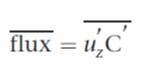
The basis for the eddy covarianve technique is that turbulent mixing, caused by the interaction of current flow with the interaction of current flow with the benthic surface, is the dominant vertical transport process in the ocean. Therefore, vertical fluxes accross the sediment-water interface can be derived from high-resolution measurements of the covariation between vertical velocity and a solute concentration. The average solute flux (C) is calculated as:
Define File Structures
First, define the input/output files to be used for each calculation.
infile = 'outfile1.dat'; %input filename with instrument counts corrected to standard units
outfile2 = 'eddyoutfile2.dat'; %output filename for fluxes (mmol m-2 h-1)and burst means
outfile3 = 'eddyoutfile3.dat'; %output filename with cumulative fluxes (mmol m-2 H-1)
outfile4 = 'outfile2O2.dat'; %O2 mean for block averaging
Set Instrument Parameters and Constants
The user must define the instrument parameters necessary to correcting for instrument geometry and sampling scheme. In this case, the EC system used a flow through pH sensor, so knowledge of the flow time through the sensor was necessary.
mheight = 0.30; % measuring height (m)
hz = 8; % frequency of measured data (Hz)
windowsize = 2401; % averaging window for running mean
B = 4; % number of bursts per hour (e.g. 15 minute bursts = 4)

% input timestamps for beginning and end of each burst
timestamps = [

13.759	13.9999
14.009	14.2499
14.259	14.4999
14.509	14.7499
14.759	14.9999
15.009	15.158
15.259	15.4999
15.509	15.7499
15.759	15.9999
16.009	16.2499
16.259	16.4999
16.509	16.7499
16.759	16.9999
17.009	17.2499
17.259	17.4999
17.509	17.7499

];
n = length(timestamps);
Import Data File
Now, import the calibrated instrument data file (defined by the variable "infile")
data = importdata(infile,' ',1); % load the data from the user defined input file

% data columns
time = data.data(:,1); % instrument time (hr)
vx = data.data(:,2); vy = data.data(:,3); vz = data.data(:,4); % velocity measurements in the x,y,z direction (ms^-1)
o2 = data.data(:,5);  % oxygen (uM)
pres = data.data(:,6); % CTD pressure measurements (dbar)
SNR = data.data(:,7); % Signal:Noise
correlation = data.data(:,8);
clear data;
Preallocate Flux Variables
% Timestamp Indices
j1 = zeros(n,1); j2 = zeros(n,1);


% Measured Parameter Variables
vxmean = zeros(n,1); vymean = zeros(n,1); vzmean = zeros(n,1);  % average velocity in the (x,y,z) directions
o2mean = zeros(n,1); % average oxygen concentration (uM)
presmean = zeros(n,1); % average CTD pressure (dbar)
SNRmean = zeros(n,1); correlationmean = zeros(n,1); % waveheight (m)
flux1o2 = zeros(n,1);  % O2 flux using method 1
flux2o2 = zeros(n,1);  % O2 flux using method 2
flux3o2 = zeros(n,1);  % O2 flux using method 3
timemean = zeros(n,1); % average time ????? why?

% Find the index of burst begin and end (using timestamps)
for i = 1:n;
    j1(i,1) = find(time > timestamps(i,1),1);
    j2(i,1) = find(time < timestamps(i,2),1,'last');
end


% Calculate means for each burst
for i = 1:n;
    timemean(i) = mean(time(j1(i):j2(i)));
    vxmean(i) = mean(vx(j1(i):j2(i)));
    vymean(i) = mean(vy(j1(i):j2(i)));
    vzmean(i) = mean(vz(j1(i):j2(i)));
    o2mean(i) = mean(o2(j1(i):j2(i)));
    presmean(i) = mean(pres(j1(i):j2(i)));
    SNRmean(i) = mean(SNR(j1(i):j2(i)));
    correlationmean(i) = mean(correlation(j1(i):j2(i)));
end


% Calculate the mean velocity (vmean) for each burst
vmean = (vxmean.^2+vymean.^2+vzmean.^2).^(1/2); % mean velocity (ms^-1)
Calculate Flux by Method #1:
%calculate fluxes by subtracting the mean for each time burst from the measurements along that time burst

vxprime1 = zeros(length(time),1);
vyprime1 = zeros(length(time),1);
vzprime1 = zeros(length(time),1);
o2prime1 = zeros(length(time),1);


for i = 1:n;
	vxprime1(j1(i):j2(i)) = vx(j1(i):j2(i))-vxmean(i);
	vyprime1(j1(i):j2(i)) = vy(j1(i):j2(i))-vymean(i);
	vzprime1(j1(i):j2(i)) = vz(j1(i):j2(i))-vzmean(i);
	o2prime1(j1(i):j2(i)) = o2(j1(i):j2(i))-o2mean(i);
	flux1primeo2 = vzprime1.*o2prime1;
	flux1o2(i) = mean(flux1primeo2(j1(i):j2(i)))*60*60;
	end
Calculate Flux by Method #2:
%calculate deviations as the residuals of the linear regression of x vs. time for each time burst

vxprime2 = zeros(length(time),1);
vyprime2 = zeros(length(time),1);
vzprime2 = zeros(length(time),1);
o2prime2 = zeros(length(time),1);
o2fit = zeros(n,2);
vxfit = zeros(n,2); vyfit = zeros(n,2); vzfit = zeros(n,2);


for i = 1:n;
	o2fit(i,:) = polyfit(time(j1(i):j2(i)),o2(j1(i):j2(i)),1);
	vxfit(i,:) = polyfit(time(j1(i):j2(i)),vx(j1(i):j2(i)),1);
	vyfit(i,:) = polyfit(time(j1(i):j2(i)),vy(j1(i):j2(i)),1);
	vzfit(i,:) = polyfit(time(j1(i):j2(i)),vz(j1(i):j2(i)),1);
	vxprime2(j1(i):j2(i)) = vx(j1(i):j2(i))-(vxfit(i,1)*time(j1(i):j2(i))+vxfit(i,2));
	vyprime2(j1(i):j2(i)) = vy(j1(i):j2(i))-(vyfit(i,1)*time(j1(i):j2(i))+vyfit(i,2));
	vzprime2(j1(i):j2(i)) = vz(j1(i):j2(i))-(vzfit(i,1)*time(j1(i):j2(i))+vzfit(i,2));
	o2prime2(j1(i):j2(i)) = o2(j1(i):j2(i))-(o2fit(i,1).*time(j1(i):j2(i))+o2fit(i,2));
	flux2primeo2 = vzprime2.*o2prime2;
	flux2o2(i) = mean(flux2primeo2(j1(i):j2(i)))*60*60;
	flux2primevx(j1(i):j2(i)) = vzprime2(j1(i):j2(i)).*vxprime2(j1(i):j2(i));
	flux2primevy(j1(i):j2(i)) = vzprime2(j1(i):j2(i)).*vyprime2(j1(i):j2(i));

end
Calculate flux by Method 3:
calculate xprime by subtracting the data smoothed by running average of size ("windowsize') from the raw data
vxprime3 = zeros(length(time),1);
vyprime3 = zeros(length(time),1);
vzprime3 = zeros(length(time),1);
o2prime3 = zeros(length(time),1);


for i = 1:n;
	vxprime3(j1(i):j2(i)) = vx(j1(i):j2(i))-smooth(vx(j1(i):j2(i)),windowsize);
	vyprime3(j1(i):j2(i)) = vy(j1(i):j2(i))-smooth(vy(j1(i):j2(i)),windowsize);
	vzprime3(j1(i):j2(i)) = vz(j1(i):j2(i))-smooth(vz(j1(i):j2(i)),windowsize);
	o2prime3(j1(i):j2(i)) = o2(j1(i):j2(i))-smooth(o2(j1(i):j2(i)),windowsize);
	flux3primeo2 = vzprime3.*o2prime3;
	flux3o2(i) = mean(flux3primeo2(j1(i):j2(i)))*60*60;
	flux3primevx(j1(i):j2(i)) = vzprime3(j1(i):j2(i)).*vxprime3(j1(i):j2(i));
	flux3primevy(j1(i):j2(i)) = vzprime3(j1(i):j2(i)).*vyprime3(j1(i):j2(i));

end
Calculate Cumulative Fluxes
cum1o2 = zeros(length(time)+n,1);
cum2o2 = zeros(length(time)+n,1);
cum3o2 = zeros(length(time)+n,1);
time1 = zeros(length(time)+n,1);

k = 1;
for i = 1:n;
    for j = j1(i):j2(i);
        if j == j1(i);
            cum1o2(k) = flux1primeo2(j);
            cum2o2(k) = flux2primeo2(j);
            cum3o2(k) = flux3primeo2(j);
            time1(k) = time(j);
            k = k+1;
        else
        time1(k) = time(j);
        sum1o2 = cum1o2(k-1)+flux1primeo2(j);
        cum1o2(k) = sum1o2;
        sum2o2 = cum2o2(k-1)+flux2primeo2(j);
        cum2o2(k) = sum2o2;
        sum3o2 = cum3o2(k-1)+flux3primeo2(j);
        cum3o2(k) = sum3o2;
        k = k+1;
        end
        if j == j2(i);
            cum1o2(k) = NaN;
            cum2o2(k) = NaN;
            cum3o2(k) = NaN;
            time1(k) = NaN;
            k = k+1;
        end
    end
end
Write Flux Calculations to Files
%Convert uMol cm L-1 s-1 at 16Hz to mmol m-2
cum1o2b = cum1o2.*0.01./hz.*B;
cum2o2b = cum2o2.*0.01./hz.*B;
cum3o2b = cum3o2.*0.01./hz.*B;

%write data to files
y1 = [timemean, vmean, o2mean, presmean, flux1o2, flux2o2, flux3o2, SNRmean, correlationmean, vxmean, vymean, vzmean];
y1 = y1';

fid1 = fopen(outfile2, 'w');


fprintf(fid1, 'timemean vmean o2mean presmean flux1o2 flux2o2 flux3o2 SNRmean correlationmean vxmean vymean vzmean \r\n');
fprintf(fid1,'%f %f %f %f %f %f %f %f %f %f %f %f \r\n', y1);
fclose(fid1);
Write Cumulative Flux Data to Files
y2 = [time1, cum1o2b, cum2o2b, cum3o2b];
k = find(time1,1,'last');
y2 = y2(1:k,:);
y2 = y2';

fid2 = fopen(outfile3, 'w');

fprintf(fid2, 'time1 cum1o2b cum2o2b  cum3o2b \r\n');
fprintf(fid2,'%f %f %f %f\r\n', y2);
fclose(fid2);