Topographic Forcing Data
Merged IBCAO/ ETOPO5 Topography
Motivation
- The recent beta release of the International Bathymetric Chart of the Arctic Ocean (IBCAO) has provided an updated, high-resolution (i.e., 2.5 km) digital topographic data base ideal for use in numerical models of the Arctic Ocean. Previously, the best available data source was the Earth-Topography-Five-Minute Gridded Elevation Data Set (ETOPO5) available at a lower resolution (i.e., 10 km).
- One difficulty with the two data sets mentioned above is that the IBCAO data is on a polar stereographic projection grid and the ETOPO5 is on a spherical coordinate grid. For use in the Arctic Ocean Model Intercomparison Project (AOMIP) the two data sets are here meshed together to form a single data set in spherical coordinates.
Meshing Details
- A FORTRAN code fragment can be used to read a data file which holds a single, direct access record containing the merged IBCAO and ETOPO5 topographic data sets.
- The merged data product resides on the same grid as the original ETOPO5 data. Since the IBCAO is at a higher resolution (i.e., ~ 2.5 km) than the ETOPO5 (i.e., ~10 km) this results in some loss of IBCAO data resolution. Nonetheless, the merged data set presented is still an improvement over the original ETOPO5 data because of the incorporation of many of the new topographic measurements that lie within the IBCAO data set.
- The merged data product has an Arctic 'focus' with no specific attention paid to the Antarctic topography. However, the Antarctic Bedmap data base will be included when publicly released.
- The merged data set is created by (i) remapping the polar stereographic projection of the original IBCAO data onto a spherical coordiante grid and (ii) merging the new spherical coordinate IBCAO grid with the ETOPO5 grid using a 'linear-ramp' weighting factor.
- The 'linear-ramp' weighting is defined such that over the southernmost 5 degree band of the IBCAO data the weights varies linearly from 1.0 to 0.0 (i.e., a 1.0 weight implies fully replacing the ETOPO5 data by the IBCAO data; a 0.0 weight implies simply taking the orginal ETOPO5 data).
- The available gzip compressed data file (TOPO_IBCAO_ETOPO5.gd.gz) is 23 MB. When gzip uncompressed the data file (TOPO_IBCAO_ETOPO5.gd) is 37 MB.
- The direct access record length of the data file is 37350724 bytes (i.e., 4 bytes per topographic value x 4321 longitudes x 2161 latitudes).
- The direct access record is read into the data array TOPO_IBCAO_ETOPO5 which has starting array index (1,1) corresponding to (longitude 0.0, latitude -90.0) and terminal array index (4321,2161) corresponding to (longitude 360.0, latitude + 90.0).
- The data array holding the topography is declared with 4 byte precision (i.e., single precision) and NOT 8 byte (i.e., double precision) because the data file is in GrADS/IEEE read/write format.
- The longitudinal and latitudinal grid spacing are exactly 1/12 of a degree everywhere on the globe (i.e. five-minutes of arc resolution).
- If you download the merged data set please let me know. If you have any difficulties using the data set or have suggestions for improving it please contact me.
Remapping IBCAO
- The objective is to exactly remap the original IBCAO data from its polar stereographic projection onto the spherical coordinate system of the earth.
- The original IBCAO data is on a right-handed Cartesian grid
 with origin at the North Pole and x-axis aligned 90 degrees counterclockwise to the direction of the prime meridian. This coordinate system has measure in units of m.
 - The IBCAO polar stereographic projection grid cuts the spherical earth along the plane intersecting the earth at latitude
 .
. - The earth's coordinate system is labeled as
 which correspond to longitude and latitude respectively. This coordinate system has measure in units of degrees.
 - The radius of the earth is taken as
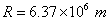 .
. - The discretization of the original IBCAO stereographic grid is 2.5 km in both x and y. The remapping creates a spherical coordinate grid having spacing of 0.10 degrees in longitude and 0.05 degrees in latitude. This new grid extends from a latitude of
 to the pole.
 - The desired topographic height
 at any point on the spherical grid is derivable from knowledge of the IBCAO topographic height
  via the coordinate transformation
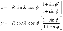
- This mapping tells us that at point
 on the original IBCAO stereographic grid we will find the desired topographic height corresponding to the point
  on the spherical grid. The quantity in square brackets is referred to as the map scale factor. Since this point
  will in general not coincide with any of the original IBCAO grids points we determine the value of
  by using interpolation over the original IBCAO grid.
 - This procedure is repeated for every point
 on the spherical grid thus completing the remapping.
 - Incidentally, performing the above coordinate transformation while ignoring the map scale factor can lead to a signifincant distortion whereby true geographical positions can be erroneously displaced by approximately 100 km. This is evident by looking at the position of the coastline (defined by the color transition from blue to green) from the merged IBCAO/ETOPO5 data as compared to the coastline (shown as white squiggly line) as taken from an accurate coastline data base. By comparison, when the maps scale factor is used there is almost an exact match between the merged IBCAO/ETOPO5 data coastline and the accurate coastline data base.
FORTRAN Code
!declare single precision local array to hold topography REAL, DIMENSION (4321,2161) :: TOPO_IBCAO_ETOPO5 !open i/o channel to data file
OPEN (UNIT = 10, & FILE ='TOPO_IBCAO_ETOPO5.gd',
& FORM ='UNFORMATTED',
& ACCESS='DIRECT',
& ACTION='READ', & RECL = 4 * 4321 * 2161)
!retrieve direct access record from data file into local array
READ (10, REC = 1) TOPO_IBCAO_ETOPO5 (:,:)


Related Files
- Descriptor File
in GrADS / ASCII control file format - Data File
gzip compressed, in GrADS / IEEE binary format
Additional Background
The recent beta release of the International Bathymetric Chart of the Arctic Ocean (IBCAO) has provided an updated, high-resolution (i.e., 2.5 km) digital topographic data base ideal for use in numerical models of the Arctic Ocean. Previously, the best available data source was the Earth-Topography-Five-Minute Gridded Elevation Data Set (ETOPO5) available at a lower resolution (i.e., 10 km). We have merged these two data sets to produce a single, high-quality global topographic data base with a high-quality representation of the arctic basin. Some details of this merged data set are as follows:
Deep Features
Here are some views of these two data sets for a Cartesian grid that spans plus-minus 20 degrees from the North Pole. Such a grid might be representative of that used in a regional model of the Arctic Basin at a 10 km model grid resolution. The color scheme is that deep blue represents -4.5 km deep and bright red represents 0.0 km. The white areas are land.
One outstanding difference between the two topographies occurs in the vicinity of the North Pole. The ETOPO5 has somewhat of a large gap in the Lomonosov ridge while the IBCAO does not. Since the ETOPO5 data was given to me second-hand (i.e., not directly from the ETOPO5 archives), I am not sure if the large gap in the Lomonosov Ridge is actually in the original ETOPO5 digital data or is an artifact of some computer processing and re-griding.
Shallow Features
To gain a better view of the shallow continental shelf areas I cut the shading range to emphasize the shallow features. The shading scheme is such that deep blue now represents -250 meters depth and bright red represents 0 m.
Difference Fields
The difference in the topographic features of the two data sets is further shown by plotting the IBCAO depths minus the ETOPO5 depths. Deep blue shading represents the IBCAO being deeper by -1.5 km or more than the ETOPO5. Bright red represents the IBCAO being shallower by 1.5 km or more than the ETOPO5.
The difference plot show a lot of bright red areas along the continental margin of the Barents, Laptev, and Kara Seas indicating that the new IBCAO data is shallower in these areas than the old ETOPO5 representation. Also, the predominance of red near the North Pole points out that the IBCAO is much shallower than the ETOPO5 in this area. This is indicative that the IBCAO has largely filled in the deep gaps seen in the ETOPO5 Lomonosov Ridge.
Lomonosov Ridge
Let's take a closer look at the bathymetric details near the Lomonosov Ridge. We will focus on a hypothetical domain that is just a 4 by 4 degree square (i.e.,. approximately 400 km on a side), centered at the North Pole. Let us take our model horizontal grid spacing relatively fine at 0.01 degree (i.e., approximately 1 km). We can compare the fine-resolution topographic realizations from the ETOPO5 and IBCAO in both a 2-D plan view and a 3-D perspective view. The 3-D view is that of an observer sitting high above the Alpha Ridge and looking 'northeastward' toward the North Pole. The observer sees the Lomonosov Ridge and somewhat obscured by the Ridge, the deep Amundsen Basin lies in the background. Also, with both the 2-D and 3-D plots the meaning of 'North' is not that consistent with a geographic map. This is because, as is common in numerical modeling of the Arctic basin, I have rotated the true geographic latitudes and longitudes by Euler Angles (0, -90,0) in order to avoid the problem of convergence of meridians near the geographic North Pole.
The two data sets differ dramatically at such fine resolution. The ETOPO5 has a large (~ 100 km) and deep (~3900 m) gap occurring in the vicinity of the North Pole. This implies that the deep waters of the Makarov and Amundsen basins could undergo uninhibited exchange down to a depth of about 3900 m when the ETOPO5 data set is used in a modeling study. By contrast. the use of the IBCAO data set would only permit exchange of water masses down to a depth of about 2500 m, and in a much narrower gap (~ 20 km). Additionally the IBCAO gap shows up as an S-shaped passageway which is located somewhat further away from the North Pole than is the gap seen in the ETOPO5 data. This IBCAO S-shape gap is also clearly visible in the recently released map of the Bottom Relief of the Arctic Ocean (All-Russian Institute for Geology and Marine Resources of the World Ocean, St. Petersburg, 1999).
Since most numerical models take a much coarser horizontal grid spacing, the above grid representation is somewhat unrepresentative of what ultimately lays at the bottom of a typical Arctic Ocean model. Let's redo the above topography but now sampling at just 0.20 degree (i.e., approximately 20 km).
It is evident that neither coarse-resolution grid can resolve the S-shape passageway that in reality exists between the Amundsen and Makarov Basins. With the ETOPO5 data set we get a very broad (~ 100 km) and deep (~3500 m) gap in the Lomonosov Ridge. The IBCAO produces a similar wide (~100 km) but somewhat shallower (~2900 m) gap. At coarse resolution the two data sets are not as great in difference as the are in fine resolution.
Another way to get a feel for the bathymetric features near the Lomonosov Ridge is to plot geopotential surfaces (i.e., at specified depths) so as to see how they intersect with the ridge. Here we plot the 3000 m, 2200 m, and 1800 m level surfaces (colored in dark blue). One way to view these surfaces is to think of them as if the ocean 'surface' was actually found at that depth horizon. In that case, the part of the ridge protruding above a given surface would in fact be 'land'. Anyway, the idea is just to illuminate that the S-shape passageway appears to be the only route for water to get between the Makarov and Amundsen Basins at depths in the range 1800 m to 2200 m. Above this depth range there is pretty much free exchange between the two basins while below this range there is no exchange.
As a simple experiment to highlight the manner in which water mass exchange might occur between the Makarov and Amundsen Basins via the S-shape gap in the Lomonosov Ridge, I run a two-layer model in the domain described above. Layer 2 is assigned as the deeper layer and it is initially permitted only to exist in (i) the Makarov Basin and (ii) only from a depth of 2200 m down to the sea floor within that basin. The idea is to have the layer 2 water in the Makarov Basin poised to spill thru the S-shape gap and on into the Amundsen Basin. Since the sill depth for the S-shape gap in the Makarov basin is approximately 2400 m, this implies that we have about 200 m worth of Makarov basin water in layer 2 that is potentially capable of spilling thru the gap. Also, layer water is present everywhere else in the domain where layer 2 water is not. We focus just on the geographical area near the gap using a 2 km model horizontal grid spacing. In the following bathymetric plot, the Makarov basin is located to the 'northwest' corner of the domain, and the Lomonosov Ridge runs along a 'southwest' to 'northeast' axis. The Amundsen Basin is located in the 'southeast' corner.
I run the 2 layer, stratified, rotating experiment for 10 simulated days. I show the initials flow velocity in layer 2, and then the subsequent flow velocities at days 5 and 10. Since this is an almost completely idealized experiment the results should only be taken in the context for which they are intended -- to qualitatively suggest the type of exchange that might occur between the two basins due to the presence of the S-shape gap.
Merged Data
An additional consideration for Arctic Ocean modeling arises from the fact that the IBCAO data only spans approximately 26 degrees of latitude from the North Pole. Model computational domains that reach further south than this require a composite topographic data set that seamlessly merges the IBCAO to the north with the ETOPO5 to the south. I have produced and made available such a merged IBCAO/ETOPO5 topographic data set by using a weighting function that appropriately blends the two data sets together.
As an example of a large model domain that would require such a merged topographic data, here is a Cartesian grid that spans plus-minus 50 degrees from the North Pole.


